
Have you guys met my friend, the scroll wheel of the mouse??
Hey everybody!
Side bar. Any Lost fans out there? For some reason, when I said hey everybody, all I could hear in my head is Charlie singing “You all everybody!”

If you’re not a Lost fan….sorry. We’ve established long before now what a nerd I am.
Annnnyway…..time for this weeks tip, and we’re sticking with Excel!
Have you ever found yourself working in Excel with a lot of data? And at the top of the columns, there are nice, organized, pretty labels for every column…..but there is SO much data, that after working for a minute, you’ve scrolled down so far that you can’t see them anymore? There’s just too. Much. INFORMATION!

Now, I’m sure none of you are like me…..thinking that I can just figure it out. I can remember the columns. Or I can just scroll up every once in awhile to refresh them in my mind. And no, I’m not mixing them up. And yes, of course I’m putting things in their right column.

However, if any of you ARE like me – let me share with you a trick I learned years ago to avoid this exact scenario.
Did you know you can freeze rows in Excel?

Luckily, it has nothing to do with Arendelle, queens or ice and everything to do with freezing the rows in place! So you can freeze the top row of your spreadsheet and no matter how much you scroll down, it will stay the top row.
Amazing. Ingenious. What will they think of next??

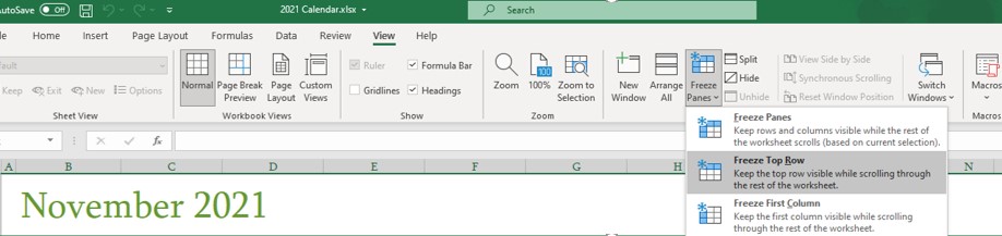
To accomplish this, just go to the View tab of Excel. Once there, you should see the Freeze Panes option which has a drop down menu. And there, you can select for it to freeze either the first row or the first column, where ever your organizational information is located.
Easy peasy lemon squeezy.
Join me next time when I teach you….ummm….more about Excel. I haven’t thought that far in advance!